Catalan Open Data exploration

import requests
import pandas as pd
import matplotlib.pyplot as plt
import matplotlib as mpl
import numpy as np

plt.style.use("../aigues-de-catalunya.mplstyle")

Data load

Agència Catalana de l’Aigua

The Agència Catalana de l’Aigua has documentation pertaining to the public APIs that allow for retrieving structured data on water in Catalonia.

Datos	Catálogo	Últimos datos recogidos
Embalses	https://aplicacions.aca.gencat.cat/sdim2/apirest/catalog?componentType=embassament	https://aplicacions.aca.gencat.cat/sdim2/apirest/data/EMBASSAMENT-EST
Aforos	https://aplicacions.aca.gencat.cat/sdim2/apirest/catalog?componentType=aforament	https://aplicacions.aca.gencat.cat/sdim2/apirest/data/AFORAMENT-EST
Pluviómetros	https://aplicacions.aca.gencat.cat/sdim2/apirest/catalog?componentType=pluviometre	https://aplicacions.aca.gencat.cat/sdim2/apirest/data/PLUVIOMETREACA-EST
Piezómetros	https://aplicacions.aca.gencat.cat/sdim2/apirest/catalog?componentType=piezometre	https://aplicacions.aca.gencat.cat/sdim2/apirest/data/PIEZOMETRE-EST

Portal de Transparència de Catalunya

Then, there is the water consumption data from the Portal de Transparència de Catalunya.

import pandas as pd
from sodapy import Socrata

# Unauthenticated client only works with public data sets. Note 'None'
# in place of application token, and no username or password:
client = Socrata("analisi.transparenciacatalunya.cat", None)

# Example authenticated client (needed for non-public datasets):
# client = Socrata(analisi.transparenciacatalunya.cat,
#                  MyAppToken,
#                  username="user@example.com",
#                  password="AFakePassword")

# First 2000 results, returned as JSON from API / converted to Python list of
# dictionaries by sodapy.
consumption_data_raw = client.get("2gws-ubmt", limit=2000)

# Convert to pandas DataFrame
consumption_data = pd.DataFrame.from_records(consumption_data_raw)

WARNING:root:Requests made without an app_token will be subject to strict throttling limits.

# normalize dtypes
consumption_data = consumption_data.astype({
    'any' : int,
    'codi_comarca' : int,
    'poblaci' : int,
    'dom_stic_xarxa' : int,
    'activitats_econ_miques_i' : int,
    'total' : int,
    'consum_dom_stic_per_c_pita' : float
})

consumption_data.head()

	any	codi_comarca	comarca	poblaci	dom_stic_xarxa	activitats_econ_miques_i	total	consum_dom_stic_per_c_pita
0	2024	1	ALT CAMP, L'	46338	1588721	2602737	4191458	93.93
1	2024	2	ALT EMPORDÀ, L'	148856	7532744	4005563	11538307	138.64
2	2024	3	ALT PENEDÈS, L'	114215	4217395	2723893	6941288	101.16
3	2024	4	ALT URGELL, L'	21214	1007067	1299444	2306511	130.06
4	2024	5	ALTA RIBAGORÇA, L'	4002	466835	429561	896396	319.59

Institut Cartogràfic i Geològic de Catalunya

The data here was obtained in the ICGC website. It refers to the geographical coordinates of the boundaries between catalan “comarques”.

import geopandas as gpd

# Path to your zipped GeoJSON file
zip_path = 'zip:///home/rcortini/work/personal_projects/aigues-de-catalunya/data/divisions-administratives-v2r1-20250101.zip!divisions-administratives-v2r1-comarques-5000-20250101.json'

# Load the GeoJSON directly from the zip
comarques = gpd.read_file(zip_path)

# Check the loaded data
comarques.head()

	CODICOMAR	NOMCOMAR	CAPCOMAR	AREAC5000	geometry
0	01	Alt Camp	Valls	537.8597	MULTIPOLYGON (((1.47594 41.47798, 1.47459 41.4...
1	02	Alt Empordà	Figueres	1356.9070	MULTIPOLYGON (((3.22338 42.23682, 3.22337 42.2...
2	03	Alt Penedès	Vilafranca del Penedès	592.5553	MULTIPOLYGON (((1.6169 41.5126, 1.61666 41.512...
3	04	Alt Urgell	la Seu d'Urgell	1446.6785	MULTIPOLYGON (((1.31941 41.99157, 1.31775 41.9...
4	05	Alta Ribagorça	el Pont de Suert	427.2234	MULTIPOLYGON (((0.8795 42.6314, 0.87928 42.631...

# some Comarca have weird names, we fix it
def fix_comarca(comarca):
    if comarca == "Moianès":
        return "MOIANÈS"
    return comarca.split(',')[0]

consumption_data['comarca_sane'] = consumption_data.comarca.apply(fix_comarca)

consumption_data

	any	codi_comarca	comarca	poblaci	dom_stic_xarxa	activitats_econ_miques_i	total	consum_dom_stic_per_c_pita	comarca_sane
0	2024	1	ALT CAMP, L'	46338	1588721	2602737	4191458	93.93	ALT CAMP
1	2024	2	ALT EMPORDÀ, L'	148856	7532744	4005563	11538307	138.64	ALT EMPORDÀ
2	2024	3	ALT PENEDÈS, L'	114215	4217395	2723893	6941288	101.16	ALT PENEDÈS
3	2024	4	ALT URGELL, L'	21214	1007067	1299444	2306511	130.06	ALT URGELL
4	2024	5	ALTA RIBAGORÇA, L'	4002	466835	429561	896396	319.59	ALTA RIBAGORÇA
...	...	...	...	...	...	...	...	...	...
540	2012	37	TERRA ALTA	12713	441824	225143	666967	95.22	TERRA ALTA
541	2012	38	URGELL, L'	36975	1543234	1422857	2966091	114.35	URGELL
542	2012	39	VAL D'ARAN, LA	10056	1112630	731409	1844038	303.13	VAL D'ARAN
543	2012	40	VALLÈS OCCIDENTAL, EL	898173	36611134	25651000	62262134	111.68	VALLÈS OCCIDENTAL
544	2012	41	VALLÈS ORIENTAL, EL	402632	17020094	14216816	31236910	115.81	VALLÈS ORIENTAL

545 rows × 9 columns

# prepare dataframes with the whole data set
df = consumption_data.drop(columns=['comarca']).rename(columns={'codi_comarca':'CODICOMAR'}).\
    drop(columns='consum_dom_stic_per_c_pita').astype({'CODICOMAR':int})
gdf = comarques.astype({'CODICOMAR':int}).merge(df, on='CODICOMAR').astype({'CODICOMAR':int}).merge(df)

Data visualizations

Industrial water consumption

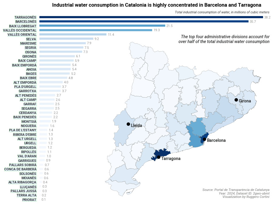
# prepare a data series for visualization. Show the cumulative distribution
s = consumption_data.query('any == 2024').set_index("comarca_sane").activitats_econ_miques_i.sort_values()
cum_s = s.cumsum()/s.sum()
cum_s.tail(10)

comarca_sane
GIRONÈS              0.323280
OSONA                0.354505
SEGRIÀ               0.386755
MARESME              0.420630
SELVA                0.460057
VALLÈS ORIENTAL      0.509066
VALLÈS OCCIDENTAL    0.591534
BAIX LLOBREGAT       0.683549
BARCELONÈS           0.836494
TARRAGONÈS           1.000000
Name: activitats_econ_miques_i, dtype: float64

fig, ax = plt.subplots(figsize=(10,8))

# 1. Normalize values
norm = mpl.colors.Normalize(
    vmin=s.min(),
    vmax=s.max()
)

# 2. Choose a colormap
cmap = mpl.cm.Blues  # we'll discuss palettes below

# 3. Map values to colors
colors = cmap(norm(s))

plot_df = s / 1e6
plot_df.plot(ax=ax, kind='barh', color=colors)

ax.set_ylabel("")
ax.tick_params(axis='both', which='both', left=False, bottom=False)
ax.set_xlabel("")
ax.set_xticklabels([])
ax.spines['left'].set_visible(False)
ax.spines['bottom'].set_visible(False)

bbox = dict(ec="limegreen", fc="xkcd:light blue", alpha=0.2, pad=0.1)
plt.setp(ax.get_yticklabels(), bbox=bbox, fontsize=8, fontweight='bold')

for i, val in enumerate(s.values):
    ax.text(val/1e6+0.2, i-0.25, f'{val/1e6:.1f}', fontsize=8, color='xkcd:grey')

ha = 0.98

ax.text(
    ha,
    1.01,
    "Total industrial consumption of water, in millions of cubic meters",
    transform=ax.transAxes,
    color='xkcd:dark grey',
    fontsize=8,
    style='italic',
    ha='right'
    )

ax.text(
    ha,
    0.02,
    "Source: Portal de Transparència de Catalunya\nYear: 2024, Dataset ID: 2gws-ubmt\nVisualization by Ruggero Cortini",
    transform=ax.transAxes,
    color='xkcd:grey',
    fontsize=8,
    style='italic',
    fontweight='medium',
    ha='right'
    )

ax.text(
    ha,
    0.85,
    "The top four administrative divisions account for\nover half of the total industrial water consumption",
    transform=ax.transAxes,
    color='xkcd:dark grey',
    fontsize=10,
    style='italic',
    fontweight='medium',
    ha='right'
    )

ax.set_title(
    "Industrial water consumption in Catalonia is highly concentrated in Barcelona and Tarragona",
    pad=20,
    fontweight='bold'
)

## MAP OF CATALONIA

# These are in unitless percentages of the figure size. (0,0 is bottom left)
left, bottom, width, height = [0.25, 0.1, 0.7, 0.7]
ax2 = fig.add_axes([left, bottom, width, height])

# prepare data to plot
plot_df = gdf.query('any == 2024')

# plot Cloropleth
plot_df.plot(
    ax=ax2,
    column='activitats_econ_miques_i',
    cmap=cmap
)

# plot contours of the Comarques
comarques.plot(
    ax=ax2,
    facecolor="none",
    edgecolor="xkcd:grey",
    linewidth=0.3
)

barcelona_coords = [2.171474, 41.389160]
girona_coords = [2.819219, 41.986706]
tarragona_coords = [1.245463, 41.116712]
lleida_coords = [0.625974, 41.617497]

city_coords = {
    'Barcelona' : barcelona_coords,
    'Girona' : girona_coords,
    'Tarragona' : tarragona_coords,
    'Lleida' : lleida_coords
}

for city, coords in city_coords.items():
    ax2.scatter(coords[0], coords[1], color='k', s=50)
    ax2.text(coords[0]+0.05, coords[1]-0.04, city, color='xkcd:dark gray', fontsize=10, fontweight='bold')

# remove spines
plt.axis('off')

fig.savefig("industrial_consumption_viz.jpg", bbox_inches='tight')
plt.show()